RCD+ server (New version 2019) is a fast loop modeling tool based on an improved version of our loop-clousureRCD method. Accurate all-atom loop predictions and ensembles can be easily generated in a few minutes for loops of 12 or less residues. Once your job is completed you can interactively check and download the predicted models.
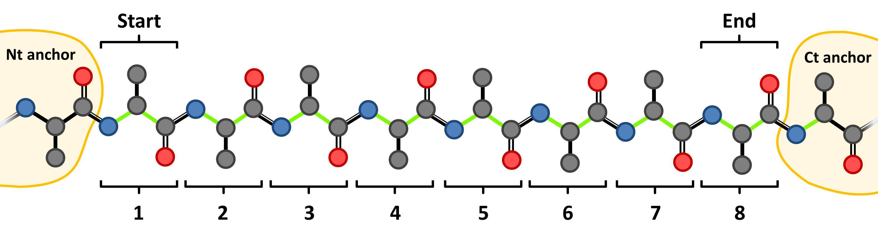
Please, upload a only protein PDB file with the atomic coordinates and introduce the following parameters: chain id, indices of the start/end residues, sequence, and select the prediction scenario between Native (if the loop environment is reliable) or Modeling (to also include the side-chains of the loop neighborhood in the refinement). The coordinates must avoid any non standard aminoacids/atoms, contain a valid chain id, and include at least the backbone of the two N- and two C-terminal anchor residues (indices Start-2, Start-1, End+1, and End+2). All residues from "Start" to "End" indices (inclusive) will be modeled from scratch.
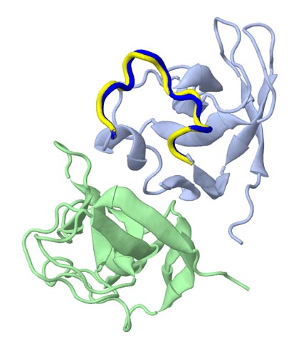
Test case: Either fetch by ID 2CMD or upload 2cmd.pdb file, and input Chain: A, Start: 270, End: 277, and Sequence: LGKNGVEE.
| *If you would like to refer our work use: | ||
| Server and improved method | López-Blanco JR, Canosa-Valls AJ, Li Y, and Chacón P (2016). RCD+: Fast loop modeling server. NAR (DOI: 10.1093/nar/gkw395).  |
|
| Original method | Chys P and Chacón P (2013). Random coordinate descent with spinor-matrices and geometric filters for efficient loop closure. J. Chem. Theory Comput. 9:1821-1829. |
|
Comparison between the loop-prediction performance of RCD+ and other state-of-the-art loop-prediction methods using the 8-residues crystallographic (Native scenario) or perturbed side-chain (Modeling scenario) test cases of the Park benchmark (Park et al. 2014 PLoS One 9:e113811).
| Nativea | Modeling | ||||||||||||||||
| PDB-ID | Residuesb | Chain | Sequence | HLPc | Galaxy | RCD+ | HLP | Galaxy | Rosetta | RCD+ | |||||||
| First | Last | Std. | PS2 | 1d | 5 | 20 | SS | PS2 | NGK | 1 | 5 | 20 | |||||
| 135l | 84 | 91 | A | LSSDITAS | 0.4 | 0.5 | 0.4 | 0.3 | 0.3 | 2.5 | 0.4 | 0.3 | 0.5 | 0.3 | 0.3 | ||
| 1alc | 34 | 41 | A | SGYDTQAI | 5.9 | 0.4 | 0.7 | 0.6 | 0.6 | 6.9 | 3.1 | 0.3 | 4.6 | 4.6 | 3.6 | ||
| 1btl | 50 | 57 | A | DLNSGKIL | 0.3 | 1.2 | 0.3 | 0.3 | 0.3 | 0.9 | 2.4 | 0.4 | 0.6 | 0.6 | 0.4 | ||
| 1cex | 73 | 80 | A | VGGAYRAT | 3.9 | 1.1 | 0.5 | 0.5 | 0.5 | 2.5 | 1.1 | 0.3 | 0.9 | 0.8 | 0.8 | ||
| 1clc | 313 | 320 | A | FRPYDPQY | 0.3 | 0.3 | 0.3 | 0.3 | 0.3 | 0.4 | 1.3 | 0.4 | 0.4 | 0.3 | 0.3 | ||
| 1ddt | 127 | 134 | A | FGDGASRV | 1.0 | 1.0 | 1.0 | 1.0 | 0.8 | 1.1 | 1.2 | 1.0 | 0.4 | 0.4 | 0.4 | ||
| 1ezm | 92 | 99 | A | GTSPLTHK | 0.4 | 0.6 | 0.3 | 0.3 | 0.3 | 0.5 | 2.5 | 0.3 | 0.4 | 0.3 | 0.3 | ||
| 1hfc | 142 | 149 | A | SNVTPLTF | 0.2 | 0.6 | 0.6 | 0.5 | 0.5 | 0.3 | 0.7 | 0.5 | 0.5 | 0.5 | 0.5 | ||
| 1iab | 48 | 55 | A | RTTESDYV | 1.6 | 1.9 | 0.5 | 0.5 | 0.4 | 0.5 | 0.7 | 0.5 | 0.5 | 0.5 | 0.5 | ||
| 1ivde | 413 | 420 | B | EGKSCINR | 0.9 | 2.9 | 1.3 | 1.0 | 1.0 | 1.3 | 3.9 | 0.8 | 1.7 | 1.7 | 1.7 | ||
| 1lst | 101 | 108 | A | PIQPTLES | 0.6 | 0.5 | 0.8 | 0.4 | 0.4 | 0.7 | 0.6 | 0.5 | 0.6 | 0.4 | 0.4 | ||
| 1nar | 192 | 199 | A | FSNQQKPV | 0.6 | 2.0 | 0.9 | 0.9 | 0.5 | 1.2 | 1.1 | 1.3 | 1.0 | 0.8 | 0.7 | ||
| 1oyc | 80 | 87 | A | GGYDNAPG | 0.5 | 0.5 | 0.3 | 0.3 | 0.3 | 0.6 | 0.4 | 0.3 | 0.4 | 0.4 | 0.4 | ||
| 1prne | 150 | 157 | A | DPDQTVDS | 1.7 | 0.5 | 0.5 | 0.3 | 0.3 | 2.3 | 0.9 | 0.3 | 0.3 | 0.3 | 0.3 | ||
| 1sbp | 107 | 114 | A | KQIHDWND | 3.3 | 0.3 | 0.3 | 0.3 | 0.3 | 0.3 | 0.4 | 0.3 | 0.4 | 0.3 | 0.3 | ||
| 1tml | 187 | 194 | A | NTSNYRWT | 0.3 | 0.9 | 0.4 | 0.3 | 0.3 | 1.5 | 1.8 | 0.5 | 0.5 | 0.4 | 0.4 | ||
| 2cmd | 270 | 277 | A | LGKNGVEE | 0.4 | 0.5 | 0.5 | 0.4 | 0.4 | 0.4 | 0.9 | 0.4 | 0.5 | 0.4 | 0.4 | ||
| 2exo | 262 | 269 | A | MQVTRCQG | 0.4 | 0.5 | 0.3 | 0.3 | 0.3 | 0.7 | 0.5 | 0.3 | 1.1 | 0.3 | 0.3 | ||
| 2sga | 8 | 15 | A | TTGGSRCS | 1.2 | 0.9 | 1.2 | 1.1 | 0.8 | 1.1 | 1.0 | 1.3 | 1.2 | 0.9 | 0.8 | ||
| 5p21 | 45 | 52 | A | VIDGETCL | 0.4 | 0.3 | 0.3 | 0.3 | 0.3 | 0.8 | 1.1 | 0.3 | 0.4 | 0.3 | 0.2 | ||
| Median | 0.6 | 0.6 | 0.5 | 0.3 | 0.3 | 0.9 | 1.1 | 0.4 | 0.5 | 0.4 | 0.4 | ||||||
| Average | 1.2 | 0.9 | 0.6 | 0.5 | 0.4 | 1.3 | 1.3 | 0.5 | 0.8 | 0.7 | 0.6 | ||||||
| Sigma | 1.5 | 0.7 | 0.3 | 0.3 | 0.2 | 1.5 | 1.0 | 0.3 | 1.0 | 1.0 | 0.8 | ||||||
| #<1Åf | 13 | 14 | 17 | 17 | 19 | 11 | 9 | 17 | 15 | 18 | 18 | ||||||
a Sampling scenarios: i) Native, the side-chains of the loop environment are kept, or ii) Modeling, include the refinement of the loop environment side-chains. In RCD+ all side-chains within 10 Å from any sampled loop Cβ were refined in the modeling scenario. The average RMSD of the lowest-energy models was computed for 9 independent RCD+ runs of the complete benchmark (all 20 cases). The RCD+ results shown correspond to the run with median value of this average.
b Residue index range, chain, and sequence of the modeled loop. The indices of the required N- and C-terminal anchor residues are First-1 and Last+1, respectively. Lowercase “p” in the sequence indicates cis-Proline.
c HLP, Rosetta, and Galaxy Root Mean Squared Deviations were taken from Table S1 of Park et al. 2014 PloS One 9:e113811 and calculated considering the main-chain atoms N, Cα, C, and O.
d RMSD of the lowest Rosetta-energy loop predicted with RCD+ together with the best RMSD of the 5 and 20 loops of lowest Rosetta-energies.
e The loops of these cases are close to neighboring oligomers, thus AB chains were considered for 1ivd and 1prn.
f Number of sub-Angstrom predictions.
Comparison between the loop-prediction performance of RCD+ and other state-of-the-art loop-prediction methods using the 12-residues crystallographic (Native scenario) or perturbed side-chain (Modeling scenario) test cases of the Park benchmark (Park et al. 2014 PLoS One 9:e113811).
| Nativea | Modeling | |||||||||||||||||
| PDB-ID | Residuesb | Chain | Sequence | HLPc | Galaxy | RCD+ | HLP | Galaxy | Rosetta | RCD+ | ||||||||
| First | Last | Std. | PS2 | 1d | 5 | 20 | SS | PS2 | NGK | NGKe | 1 | 5 | 20 | |||||
| 1a8d | 155 | 166 | A | DLPDKFNAYLAN | 1.0 | 0.3 | 0.8 | 0.8 | 0.8 | 2.7 | 0.5 | 5.2 | 0.4 | 5.2 | 1.1 | 1.1 | ||
| 1arb | 182 | 193 | A | WQPSGGVTEPGS | 2.5 | 2.0 | 0.7 | 0.7 | 0.7 | 1.0 | 1.0 | 0.4 | 1.3 | 1.4 | 0.7 | 0.7 | ||
| 1bhe | 121 | 132 | A | GQGGVKLQDKKV | 0.5 | 1.0 | 2.2 | 2.2 | 2.2 | 0.5 | 2.0 | 0.4 | 0.4 | 0.8 | 0.8 | 0.8 | ||
| 1bn8 | 298 | 309 | A | STSSSSYPFSYA | 1.5 | 0.7 | 0.7 | 0.7 | 0.7 | 1.3 | 1.6 | 1.1 | 1.3 | 0.5 | 0.5 | 0.5 | ||
| 1c5ef | 82 | 93 | A | YEDVLWPEAASD | 0.4 | 1.6 | 0.4 | 0.4 | 0.4 | 0.4 | 0.5 | 0.4 | 0.4 | 0.6 | 0.4 | 0.4 | ||
| 1cb0 | 33 | 44 | A | YVDTPFGKPSDA | 0.3 | 0.5 | 0.4 | 0.4 | 0.4 | 0.3 | 0.5 | 0.6 | 0.5 | 0.5 | 0.4 | 0.4 | ||
| 1cnv | 188 | 199 | A | FYNDRSCQYSTG | 2.2 | 2.5 | 3.3 | 2.7 | 1.4 | 1.5 | 3.2 | 2.0 | 1.7 | 3.8 | 1.9 | 1.9 | ||
| 1cs6 | 145 | 156 | A | NEFpNFIPADGR | 0.6 | 3.6 | 4.1 | 4.1 | 3.5 | 1.6 | 3.1 | 2.5 | 4.0 | 4.2 | 4.1 | 4.0 | ||
| 1dqz | 209 | 220 | A | CGNGTPSDLGGD | 0.3 | 0.7 | 0.4 | 0.4 | 0.4 | 0.7 | 1.0 | 0.6 | 0.5 | 1.0 | 0.9 | 0.8 | ||
| 1exm | 291 | 302 | A | RGVSREEVERGQ | 0.7 | 1.2 | 0.5 | 0.5 | 0.5 | 4.5 | 1.2 | 1.0 | 0.6 | 0.6 | 0.4 | 0.4 | ||
| 1f46 | 64 | 75 | A | MVKpGTFDPEMK | 0.3 | 1.6 | 0.4 | 0.4 | 0.3 | 0.5 | 1.5 | 2.1 | 3.3 | 0.6 | 0.4 | 0.4 | ||
| 1i7p | 63 | 74 | A | LPSPQHILGLPI | 0.3 | 0.3 | 0.3 | 0.3 | 0.3 | 0.3 | 0.3 | 0.4 | 2.6 | 0.4 | 0.3 | 0.3 | ||
| 1m3sf | 68 | 79 | A | VGEILTPPLAEG | 5.0 | 6.0 | 0.8 | 0.4 | 0.4 | 5.1 | 5.9 | 6.4 | 5.6 | 0.5 | 0.3 | 0.3 | ||
| 1ms9 | 529 | 540 | A | GSTPVTPTGSWE | 1.9 | 1.3 | 0.3 | 0.3 | 0.3 | 2.8 | 2.6 | 2.7 | 1.3 | 0.3 | 0.3 | 0.3 | ||
| 1my7 | 254 | 265 | A | TPPYADPSLQAP | 0.5 | 2.6 | 0.4 | 0.4 | 0.4 | 0.9 | 2.9 | 0.6 | 0.6 | 0.6 | 0.6 | 0.6 | ||
| 1oth | 69 | 80 | A | QKGEYLPLLQGK | 1.8 | 0.5 | 2.2 | 2.2 | 0.5 | 0.5 | 2.3 | 0.4 | 0.4 | 1.5 | 0.8 | 0.8 | ||
| 1oyc | 203 | 214 | A | DPHSNTRTDEYG | 0.5 | 2.1 | 0.7 | 0.6 | 0.6 | 0.5 | 1.4 | 0.4 | 0.9 | 4.6 | 0.8 | 0.7 | ||
| 1qlwf | 31 | 42 | A | ETLSLSPKYDAH | 1.9 | 1.5 | 0.5 | 0.4 | 0.4 | 2.0 | 4.6 | 4.8 | 0.7 | 0.7 | 0.6 | 0.5 | ||
| 1t1d | 127 | 138 | A | SGGRLRRPVNVP | 0.5 | 1.6 | 0.4 | 0.4 | 0.4 | 0.8 | 1.0 | 0.7 | 0.8 | 0.4 | 0.4 | 0.4 | ||
| 2pia | 30 | 41 | A | DPQGAPLPPFEA | 0.6 | 0.8 | 1.0 | 0.4 | 0.3 | 0.5 | 5.5 | 0.8 | 0.9 | 0.6 | 0.6 | 0.4 | ||
| Median | 0.6 | 1.4 | 0.6 | 0.4 | 0.4 | 0.9 | 1.6 | 0.8 | 0.8 | 0.6 | 0.6 | 0.5 | ||||||
| Average | 1.2 | 1.6 | 1.0 | 0.9 | 0.7 | 1.4 | 2.1 | 1.7 | 1.4 | 1.4 | 0.8 | 0.8 | ||||||
| Sigma | 1.2 | 1.3 | 1.1 | 1.0 | 0.8 | 1.4 | 1.7 | 1.8 | 1.4 | 1.6 | 0.9 | 0.9 | ||||||
| #<1Åg | 12 | 7 | 16 | 16 | 17 | 11 | 4 | 11 | 12 | 13 | 17 | 17 | ||||||
a Sampling scenarios: i) Native, the side-chains of the loop environment are kept, or ii) Modeling, include the refinement of the loop environment side-chains. In RCD+ all side-chains within 10 Å from any sampled loop Cβ were refined in the modeling scenario. The average RMSD of the lowest-energy models was computed for 9 independent RCD+ runs of the complete benchmark (all 20 cases). The RCD+ results shown correspond to the run with median value of this average.
b Residue index range, chain, and sequence of the modeled loop. The indices of the required N- and C-terminal anchor residues are First-1 and Last+1, respectively. Lowercase “p” in the sequence indicates cis-Proline.
c HLP, Rosetta, and Galaxy Root Mean Squared Deviations were taken from Table S2 of Park et al. 2014 PLoS One 9:e113811 and calculated considering the main-chain atoms N, Cα, C, and O.
d RMSD of the lowest Rosetta-energy loop predicted with RCD+ together with the best RMSD of the 5 and 20 loops of lowest Rosetta-energies.
e These NGK results were taken from NGK's paper (Stein and Kortemme 2013 PLoS One 8(5):e63090).
f The loops of these cases are close to neighboring oligomers, thus AB chains were considered for 1c5e and 1qlw, and ABCD for 1m3s.
g Number of sub-Angstrom predictions.
Results obtained with different strategies to enrich the RCD sampling in near-native conformations. The 8 and 12 residues cases of three standard benchmarks were used: Canutescu (Canutescu and Dunbrack 2003 Protein Science 12:963), Soto (Soto et al. 2008 Proteins 70:834), and Park (Park et al. 2014 PLoS One 9:e113811). In all the cases, unless otherwise stated, 5000 loops were generated using randomly perturbed standard bond angles and lengths.
CANUTESCU's benchmark
| 8 residues (10 cases) | 12 residues (10 cases) | |||||||||||||||||||||
| Filtera | RMSDb [Å] | <0.5c | <1.0 | <1.5 | <2.0 | <2.5 | <3.0 | Timed | RMSD [Å] | <0.5 | <1.0 | <1.5 | <2.0 | <2.5 | <3.0 | Time | ||||||
| Min | Avg | σ | [%] | [%] | [%] | [%] | [%] | [%] | [ms] | Min | Avg | σ | [%] | [%] | [%] | [%] | [%] | [%] | [ms] | |||
| None | 1.45 | 4.78 | 1.32 | 0.00 | 0.00 | 0.02 | 0.54 | 3.91 | 12.49 | 0.8 | 2.21 | 6.66 | 1.67 | 0.00 | 0.00 | 0.00 | 0.01 | 0.13 | 0.98 | 1.1 | ||
| Simple | 1.39 | 4.49 | 1.21 | 0.00 | 0.01 | 0.17 | 1.47 | 6.60 | 15.77 | 6.1 | 2.16 | 6.29 | 1.53 | 0.00 | 0.00 | 0.00 | 0.00 | 0.17 | 1.09 | 3.2 | ||
| Dunbrack | 0.79 | 4.18 | 1.27 | 0.00 | 0.19 | 1.14 | 4.27 | 12.19 | 24.05 | 1.2 | 1.62 | 5.92 | 1.71 | 0.00 | 0.00 | 0.02 | 0.29 | 1.42 | 4.06 | 5.1 | ||
| +Bumps+ICOSAe | 0.68 | 3.34 | 0.96 | 0.01 | 1.17 | 5.63 | 14.50 | 29.31 | 44.80 | 32 | 1.31 | 4.51 | 1.27 | 0.00 | 0.01 | 0.34 | 2.46 | 8.13 | 17.25 | 115 | ||
a Methods used to enrich RCD sampling in near-native conformations. None: RCD. Simple: Simplified Ramachandran filter of the old RCD version. Dunbrack: Detailed Neighbor-dependant Ramachandran filter. +Bumps+ICOSA: Clash and Energy filters applied after Dunbrack filter.
b Minimum, Average, and Sigma of the Root Mean Squared Deviations calculated using N,Cα,C,O atoms.
c Percentage of loops below indicated RMSD.
d Average time to generate a single loop using 14 cores of two Intel Xeon E5-2650 CPUs (2.00GHz).
e In this case, the top 5000 loops with best ICOSA energy were selected from a 50K bump-free sampling.
SOTO's benchmark
| 8 residues (49 cases) | 12 residues (10 cases) | |||||||||||||||||||||
| Filter | RMSD [Å] | <0.5 | <1.0 | <1.5 | <2.0 | <2.5 | <3.0 | Time | RMSD [Å] | <0.5 | <1.0 | <1.5 | <2.0 | <2.5 | <3.0 | Time | ||||||
| Min | Avg | σ | [%] | [%] | [%] | [%] | [%] | [%] | [ms] | Min | Avg | σ | [%] | [%] | [%] | [%] | [%] | [%] | [ms] | |||
| None | 1.46 | 4.48 | 1.59 | 0.00 | 0.00 | 0.09 | 1.71 | 7.73 | 18.53 | 1.2 | 2.24 | 6.72 | 1.73 | 0.00 | 0.00 | 0.00 | 0.00 | 0.11 | 0.64 | 0.9 | ||
| Simple | 1.30 | 4.23 | 1.47 | 0.00 | 0.01 | 0.63 | 3.15 | 9.14 | 20.52 | 33 | 2.27 | 6.44 | 1.62 | 0.00 | 0.00 | 0.00 | 0.01 | 0.14 | 0.96 | 2.8 | ||
| Dunbrack | 0.78 | 3.51 | 1.42 | 0.00 | 0.70 | 4.79 | 13.36 | 25.85 | 40.25 | 1.5 | 1.68 | 5.90 | 1.71 | 0.00 | 0.00 | 0.04 | 0.30 | 1.37 | 3.98 | 3.0 | ||
| +Bumps+ICOSA | 0.84 | 3.02 | 0.88 | 0.02 | 2.90 | 11.64 | 25.66 | 41.44 | 56.50 | 33 | 1.34 | 4.67 | 1.03 | 0.00 | 0.01 | 0.42 | 2.44 | 8.10 | 16.96 | 69 | ||
* See Canutescu's table foot notes.
PARK's benchmark
| 8 residues (20 cases) | 12 residues (20 cases) | |||||||||||||||||||||
| Filter | RMSD [Å] | <0.5 | <1.0 | <1.5 | <2.0 | <2.5 | <3.0 | Time | RMSD [Å] | <0.5 | <1.0 | <1.5 | <2.0 | <2.5 | <3.0 | Time | ||||||
| Min | Avg | σ | [%] | [%] | [%] | [%] | [%] | [%] | [ms] | Min | Avg | σ | [%] | [%] | [%] | [%] | [%] | [%] | [ms] | |||
| None | 1.50 | 5.35 | 1.92 | 0.00 | 0.00 | 0.02 | 0.45 | 3.21 | 8.92 | 0.6 | 2.19 | 6.81 | 2.16 | 0.00 | 0.00 | 0.00 | 0.07 | 0.91 | 3.18 | 2.4 | ||
| Simple | 1.29 | 5.13 | 1.87 | 0.00 | 0.00 | 0.14 | 1.08 | 4.99 | 12.98 | 1.8 | 2.12 | 6.57 | 2.08 | 0.00 | 0.00 | 0.00 | 0.05 | 0.66 | 2.98 | 9.5 | ||
| Dunbrack | 0.84 | 4.17 | 1.78 | 0.00 | 0.44 | 3.42 | 9.87 | 18.66 | 28.64 | 1.4 | 1.50 | 5.64 | 1.97 | 0.00 | 0.02 | 0.40 | 2.29 | 6.48 | 12.89 | 4.6 | ||
| +Bumps+ICOSA | 0.67 | 3.10 | 0.95 | 0.01 | 3.52 | 14.98 | 27.17 | 40.19 | 53.14 | 33 | 1.19 | 4.31 | 1.24 | 0.00 | 0.16 | 1.93 | 7.44 | 17.07 | 28.76 | 116 | ||
* See Canutescu's table foot notes.
Minimum RMSD (RMSDmin) obtained with different loop-closure algorithms. In all the cases, 5000 loops were generated using two classical loop modeling benchmarks, Canutescu (Canutescu and Dunbrack 2003 Protein Science 12:963) and Soto (Soto et al. 2008 Proteins 70:834), and compared with the native conformation.
Sampling comparison between RCD+ and other methods using Canutescu's data set
| RMSDmina [Å] | |||
| Algorithm | 4 residues | 8 residues | 12 residues |
| CCD | 0.56 | 1.59 | 3.05 |
| CJSD | 0.40 | 1.01 | 2.34 |
| SOS | 0.20 | 1.19 | 2.25 |
| FALCm | 0.22 | 0.72 | 1.81 |
| DiSGro | 0.21 | 0.80 | 1.53 |
| RCD | 0.28 | 0.81 | 1.59 |
| RCD+ | 0.17 | 0.71 | 1.63 |
| RCD+b | 0.27 | 0.79 | 1.62 |
a Averages of the minimum backbone RMSD over 5000 loops generated for each of the 10 test cases of Canutescu's benchmark (Canutescu and Dunbrack 2003 Protein Science 12:963). RCD values were taken from Table 2 of Chys and Chacón 2013 9:1821, and the others from.
b In this case, loops were generated using randomly perturbed standard bond angles and lengths whereas in all the other algorithms native bond angles and lengths were employed instead.
Sampling comparison between RCD+ and other methods using Soto's data set
| RMSDmina [Å] | |||
| Algorithm | 8 residues | 11 residues | 12 residues |
| (49 cases) | (17 cases) | (10 cases) | |
| Random tweak | 1.22 | 2.22 | 2.64 |
| CCD | 1.20 | 2.11 | 2.57 |
| Wriggling | 1.43 | 2.24 | 2.68 |
| PLOP-build | 0.99 | 2.18 | 2.69 |
| Direct tweak | 0.69 | 1.20 | 1.48 |
| LOOPYbb | 0.89 | 1.51 | 1.80 |
| DiSGro | 0.80 | 1.19 | 1.28 |
| RCD | 0.78 | 1.38 | 1.60 |
| RCD+ | 0.64 | 1.28 | 1.56 |
| RCD+b | 0.78 | 1.33 | 1.68 |
a Averages of the minimum backbone RMSD over 5000 generated loops using the Soto's benchmark (Soto et al. 2008 Proteins 70:834). RCD values were taken from Table 3 of Chys and Chacón 2013 9:1821, and the others from Table 2 of Soto et al. 2008 Proteins 70:834.
b In this case, loops were generated using randomly perturbed standard bond angles and lengths whereas in all the other algorithms native bond angles and lengths were employed instead.
Despite the results are reported on the same benchmark sets, loops were modeled under different assumptions. For example, the number of atoms (or degrees of freedom) effectively modeled vary depending of the algorithm. Many of the classical methods retained the native bond angles and lengths. It is also frequent to exclude the N and Cα atoms of the first loop residue from the modeling and/or the Cα and C atoms of the last loop residue. There are also slight variations in the RMSD criteria: there are methods that calculate the RMSD with the main-chain atoms N, Cα, and C, while others also include the O atom. Our RCD+ results are reported including the O atom in the RMSD and using the most challenging and realistic assumptions: 1) we do not use any information from the native loop (bond angles and lengths are modeled from scratch), and 2) we modelled the complete loop from the first residue to the last, i.e. the anchor residues (fixed) are outside the modeled region.
In any case, as it can be seen, RCD+ yields very competitive results. The average RMSDmin is significantly lower than in other methods with the exception of DiSGro. Nevertheless, DiSGro considers less atoms in the modeling because it requires the N and Cα atoms of the first loop residue and the Cα and C atoms of the last; our RCD+ does not, effectively modeling all the atoms of the loop.
Loop generation stage of RCD+ has been parallelized by MPI. Below, the experimental average time (blue) to generate one 12-residues loop is compared with the theoretical expected time (red) for different number of processing cores in our dual Intel Xeon E5-2650 server (2.00GHz).

*5000 loops were generated using the neighbor-dependent Ramachandran filter and randomly perturbed standard bond angles and lengths with the Park benchmark (Park et al. 2014 PLoS One 9:e113811).
Feel free to explore (or submit again) any of the precomputed examples for the Modeling scenario!
 Malate dehydrogenase (2CMD:A, A270-277) (8-residues) INPUT: ID= 2CMD:A, Chain= A, Start= 270, End= 277, Modeling |
 λ-phage head protein D (1C5E:AB, A82-93) (12-residues) INPUT: ID= 1C5E:AB, Chain= A, Start= 82, End= 93, Modeling |
 TEM1 beta-lactamase (1BTL:A, A50-57) (8-residues) INPUT: ID= 1BTL:A, Chain= A, Start= 50, End= 57, Modeling |
 Shaker K+ channel T1 (1T1D:A, A127-138) (12-residues) INPUT: ID= 1T1D:A, Chain= A, Start= 127, End= 138, Modeling |
 Chitinase (Homology Model 1D2K:A, A349-354) (6-residues) INPUT: ID*= 1D2K:A, Chain= A, Start= 349, End= 354, Modeling *Homology Model taken from Seok's benchmark. |
 Serratia protease (1SRP:A, A311-322) (12-residues) INPUT: ID= 1SRP:A, Chain= A, Start= 311, End= 322, Modeling |
 Rac1-SptP complex (1G4U:RS, R30-39) (10-residues) INPUT: ID= 1G4U:RS, Chain= R, Start= 30, End= 39, Modeling |
 Rac1-RhoGDI complex (1HH4:AD, A30-39) (10-residues) INPUT: ID= 1HH4:AD, Chain= A, Start= 30, End= 39, Modeling |
 Antibody H3 loop (1FGN:HL, H99-106) (8-residues) INPUT: ID= 1FGN:HL, Chain= H, Start= 99, End= 106, Modeling |
 Antigen-Antibody H3 loop (2BDN:AHL, H99-106) (8-residues) INPUT: ID= 2BDN:AHL, Chain= H, Start= 99, End= 106, Modeling |
- Introduction.
RCD+ method - Step 1.
Basic input - Step 2. (optional)
Advanced options - Step 3.
Queue - Step 4.
Explore results - Step 5. (optional)
Download results
The improved version of the Random Coordinate Descent (RCD) algorithm is used to generate an ensemble of closed loops (up to 50K in the server) by rotation of the φ and ψ backbone dihedral angles according to detailed neighbor-dependent Ramachandran probability distributions:

Upon loop closure, the loops are evaluated using a fast coarse-grained energy function (ICOSA) and then the best 10% is selected. Finally, these lowest-scoring models are further refined using a detailed energy function (Rosetta) to obtain accurate all-atom predictions.
To perform such loop predictions you only need a minimal basic input: the atomic coordinates of the environment (PDB-file or fetch from PDB) and the boundary residue indices, sequence, and chain of the loop (Step 1). When you press the submit button you will check the job status in the queue tab (Step 3). Once job run is completed you can interactively explore the predicted models in the results tab (Step 4) and/or download them (Step 5). Optionally, advanced users are encouraged to customize RCD+ run by tuning the parameters in the advanced options panel (Step 2).
Please, introduce the following required data and then click on the submit button to perform the predictions:

(1) Upload your protein atomic structure in PDB format (v3.x) or fetch it by PDB-ID. It is mandatory to follow the PDB format avoiding non standard aminoacids (eg. no CYX, HIE etc.) and atom names. The presence of chain ID is also mandatory. The vast majority of RCD malfunctioning is due to format errors in the PDB. The fetching input format is ID:Chain(s) (In case you don't introduce any chain ID, the first chain ID found in PDB file will be considered). The fetching is very customizable. For example, introduce:
2CMD:A to use the A chain from 2CMD entry,
2BDN:HL to consider the antibody chains H and L of this antigen/antibody complex, or
2BDN:AHL to consider the antigen as well (chain A).
IMPORTANT: This structure will define the loop environment for clash detection and provide the coordinates of anchor aminoacids.
(2) Introduce the chain ID and the Start (first) and End (last) residue indices of the loop. Note that these terminal residues are modeled from scratch and only the N- and C-terminal anchors (indices Start-1 and End+1) and their neighboring residues (indices Start-2 and End+2) are required, e.g. for a 8 residues loop:
A and 270-277 for 2CMD entry or
H and 99-106 for the antigen/antibody case.
(More examples of different loop lengths are provided in the Gallery tab.)
(3) Choose a prediction scenario:
Native if the side-chain conformations of the loop neighborhood are reliable, e.g. building a chrystallographic missing loop or
Modeling to also include the side-chains of the loop neighborhood in the refinement, e.g. predicting loops in homology modeling. As a rule of thumb, Modeling predictions take around three times longer than Native predictions.
(4) Type or paste the sequence of the modeled loop in one letter format (not including anchor aminoacids). This will be the sequence of all modeled loops. Alternatively, leave this field blank to automatically get the sequence from PDB coordinates. Introduce these sequences for the examples:
LGKNGVEE for 2CMD case or
GVFGFFDY for the antigen/antibody complex.
(4) We optionally encourage you to introduce some descriptive job name and an email address for quick results identification and access. It is highly recomended that you use the JAVA interface (JSmol box) in case you have a JAVA virtual machine enabled in the browser since the best 3D visualization performance is only achieved with JAVA. Note that this is not the same as having JavaScript activated. To maximize compatibility with all browsers and devices (Android, iPad or iPhone), please, use HTML5 interface instead (by default).

If you are an advanced user, you may want to change default RCD+ parameters. Please, click the "+" to deploy the advanced options:
- Number of closed loops generated (#Loops): By default, a different number of loops is sampled depending on the loop length, but other values within 1K-50K range can be selected. For example, while for 8 residues loops 5K loops are usually enough to obtain sub-angstrom predictions, for 12 residues higher values may be required (10-50K).
- Number of closed loops to be refined (#ICOSA): Number of loops with lowest coarse-grained ICOSA energy that will be all-atom refined in Rosetta.
- Ramachandran threshold (%Rama): This is the percentage of probability that defines the allowed regions of the Ramachandran maps used to constrain the conformational search [Ting et al. (2010)]. The default value depends on loop length and produces good results, but it can be tuned in the range [80-99.99%] to obtain better (or worse) results. You will see the effect that such changes produce in the shaded regions of Ramachandran maps once results have been computed.
- Atomic model: Four different atomic models can be selected for clash detection in the conformational search stage: (N,Cα,C), (N,Cα,C,O), (N,Cα,C,Cβ), and the most detailed (N,Cα,C,O,Cβ). Only the indicated atoms will be considered in this stage. Note that all-atom loops will be generated and considered later in the refinement stage.
- RCD method: The neighbor-dependent Ramachandran filter of the improved RCD method (Dunbrack) is the default option, but you can select the original simplified method (Simple) or an unconstrained version (Free) as well.
Any option available in the RCD standalone program can be added in the expert options box. Note that a maximum wall-time of 1 hour per job has been set to prevent abuse.
Inmediately upon job submission, your job will be queued in our server and you will be redirected to Queue status tab. In this tab all jobs submited to RCD+ Server are listed. Your jobs are shown in darker colors whereas those submitted by others appear in lighter colors. You can check server usage and whether any queued job is running ("r" status, green) or queued ("qw" status, orange). In case any of your jobs has been queued ("qw" status) it will run as soon as computational resources become available.

Once a standard-sized job is running ("r" status) it usually takes around 10-15 minutes to complete depending on its size. For example, the modeling of a large loop (12-residues) usually takes around 10 minutes. To avoid server overloading the wall-time of Native and Modeling jobs has been set to 2 and 4 hours, respectively.

As soon as your jobs finish they will move to the list of "Your finished jobs" for further access and a direct link will appear to redirect you to the Results of the last finished job.

In case you detect any problem in any of your submitted jobs they can be easily deleted by clicking the corresponding red cross. A "dr" status (black) will evidence that it is being deleted from queue. Note that anyone but you can delete your jobs.
Please, do not close the browser unless you have either kept track of the job ID or provided an email address, otherwise you will not be able to access your results when the web browser is closed.
Use mouse controls to interactively explore the generated loops in JSmol and customize their molecular representation and colors. For example, just drag for rotating, hold Shift key + double click for translating, or click in the palette to change the color of the selected loop(s). The user can choose between three different interfaces: Java, HTML5 and WebGL. The HTML5-javascript interface is activated by default. To activate the JAVA, first you must enable it in your web browser (details) and add frodock.chaconlab.org to the exception sites in the Java panel (details).

You can also check the structural qualitiy of the generated loops by deploying the More information section.

Only if you included the native loop in the PDB (just for benchmarking purposes) the result error in RMSD is evaluated and plotted versus the loop energy for all loop models.

Finally, all computed results are freely avaible for download:

- All refined loops: All-atom refined models as a single Multi-PDB file.
- All closed loops: All closed loop models produced by RCD+ (before any Rosetta refinement) at selected Coarse-Graining level (a single Multi-PDB file too).
- Dunbrack plots: Neighbor-dependent Ramachandran maps, dihedral angles, and images are provided as plain text or JPG images.
- Energy evaluation: Refinement summary table for all refined loops (plain text file) with the loop indices (#loop), the all-atom Rosetta energy before any refinement for the full protein (E_full) and the loop (E_loop), the all-atom Rosetta energy after refinement (E_full2), the RMSDs before (before E_full2 column) and after (after E_full2 column) refinement considering N,Cα,C,O atoms (R_rcd and R_BBO), N,Cα,C (R_BB), all heavy atoms (R_HA), all side-chain heavy atoms (R_SC), and all atoms including hydrogens (R_ALL).
- Summary results: RCD+'s output summary.
- Log-file: Plain text log file with the start/end time for each of the protocol steps.
- All computed files: A tar+gzip file containing all job data.